Example: Two Region Fit in NGC 628#
This notebook outlines a similar procedure as followed in Lehmer et al. (2024) to fit the SFHs of galaxies in two regions, using NGC 628 as an example.
Briefly, the central regions of spiral galaxies suffer from crowding in Chandra imaging, preventing us from counting individual X-ray, such that the X-ray binary luminosity function can only be constructed outside the central region. In Lehmer et al. (2024), where our goal was to connect the XLF to the SFH of the galaxy, this meant that we needed to exclude the center of many galaxies from the estimation of the SFH. However, deriving the SFH by fitting only the SED of the outer region would force us to ignore IR data which does not resolve the separate regions. To preserve the valuable IR constraints on the SFH, we hacked together this method for jointly fitting the central and outer regions of the galaxy, such that the sum of the two SED models is constrained by the IR measurements.
Imports#
[1]:
import h5py
import sys
from pprint import pprint
import numpy as np
from astropy.table import Table

from lightning import Lightning
from lightning.priors import UniformPrior
from multi_lightning import MultiLightning
from multi_lightning.priors import FixedConnection, NormalConnection, UniformConnection

import corner
import matplotlib.pyplot as plt

%matplotlib inline
Read data and construct flux arrays#
[2]:
phot = Table.read('NGC0628-photometry.fits')

filter_labels = np.array([s.strip() for s in phot['FILTER_LABELS']])
filter_labels[filter_labels == ['2MASS_K']] = '2MASS_Ks'

Nfilters = len(filter_labels)

#ascii.write(phot['FILTER_LABELS','WAVELENGTH'], format='fixed_width_two_line')

fnu = phot['FNU_OBS'] * 1e3 # in mJy
fnu_cent = phot['FNU_CENT_OBS'] * 1e3 # in mJy
# By the construction of this catalog, the annulus photometry is the difference of the total and center regions.
fnu_out = fnu - fnu_cent


# For this example we assume that the uncertainty in the flux is
# dominated by the absolute flux calibration, and we ignore the
# background.
cal_unc = np.array([0.15, 0.15, # GALEX
                    0.05, 0.05, 0.05, 0.05, 0.05, # SDSS
                    0.05, 0.05, 0.05, # 2MASS
                    0.05, 0.05, 0.05, 0.05, # IRAC
                    0.05, # MIPS 24 um
                    0.05, 0.05, 0.05, # PACS
                    0.15, 0.15, 0.15, # SPIRE
                    0.07, 0.07, 0.07, 0.07 # WISE
                    ])

fnu_unc = cal_unc * fnu
fnu_out_unc = cal_unc * fnu_out
fnu_cent_unc = cal_unc * fnu_cent

fnu_unc = cal_unc * fnu
fnu_out_unc = cal_unc * fnu_out
fnu_cent_unc = cal_unc * fnu_cent

unresolved = (fnu != 0) & (fnu_cent == 0)
resolved = ~unresolved

fnu[fnu == 0] = np.nan
fnu_out[fnu_cent == 0] = np.nan
fnu_cent[fnu_cent == 0] = np.nan

# The flux array has Nregions+1 rows, where the extra (first) row
# corresponds to the "total" fluxes, from the bands that
# do not resolve the regions.
fnu_arr = np.zeros((3, Nfilters))
fnu_arr[1,:] = fnu_cent
fnu_arr[2,:] = fnu_out
fnu_arr[0,unresolved] = fnu[unresolved]
fnu_arr[0,resolved] = np.nan

# Likewise for the uncertainty array.
fnu_unc_arr = np.zeros((3, Nfilters))
fnu_unc_arr[1,:] = fnu_cent_unc
fnu_unc_arr[2,:] = fnu_out_unc
fnu_unc_arr[0,unresolved] = fnu_unc[unresolved]
fnu_unc_arr[0,resolved] = 0.0
Initialize the Lightning and MultiLightning Objects#
Things to notice: - The first positional argument for MultiLightning is itself a Lightning object or list of objects defining the models to use for each region. - Here, we only need to define one Lightning object, since we use the same model for both regions. In some scenarios you can imagine having different models, for example if you need to include an AGN component in the nuclear region.
[3]:
reg_names = ['center', 'disk']

redshift = 0.0
DL = 7.3 # Mpc - collected from Moustakis+2010, originally measured by Sharina+(1996) from supergiant stars.

lgh = Lightning(filter_labels,
                lum_dist=DL,
                atten_type='Calzetti',
                dust_emission=True)

# lgh.save_json('NGC0628_config.json')


mlgh = MultiLightning(lgh,
                      fnu_arr,
                      fnu_unc_arr,
                      model_unc=0.10,
                      Nregions=2,
                      reg_names=reg_names)

print('Priors are still given as ordered lists, so it is useful to use `print_params` to see what that order should be.')
lgh.print_params(verbose=True)
Priors are still given as ordered lists, so it is useful to use `print_params` to see what that order should be.

============================
Piecewise-Constant
============================
Parameter  Lo  Hi              Description
--------- --- --- ------------------------
    psi_1 0.0 inf SFR in stellar age bin 1
    psi_2 0.0 inf SFR in stellar age bin 2
    psi_3 0.0 inf SFR in stellar age bin 3
    psi_4 0.0 inf SFR in stellar age bin 4
    psi_5 0.0 inf SFR in stellar age bin 5

============================
Pegase-Stellar
============================
Parameter    Lo  Hi                                      Description
--------- ----- --- ------------------------------------------------
     Zmet 0.001 0.1 Metallicity (mass fraction, where solar = 0.020)

============================
Calzetti
============================
     Parameter  Lo  Hi                      Description
-------------- --- --- --------------------------------
calz_tauV_diff 0.0 inf Optical depth of the diffuse ISM

============================
DL07-Dust
============================
      Parameter     Lo       Hi                                                             Description
--------------- ------ -------- -----------------------------------------------------------------------
dl07_dust_alpha  -10.0      4.0                  Radiation field intensity distribution power law index
dl07_dust_U_min    0.1     25.0                                       Radiation field minimum intensity
dl07_dust_U_max 1000.0 300000.0                                       Radiation field maximum intensity
dl07_dust_gamma    0.0      1.0 Fraction of dust mass exposed to radiation field intensity distribution
dl07_dust_q_PAH 0.0047   0.0458                            Fraction of dust mass composed of PAH grains

Total parameters: 12
Fit the model#
[4]:
# This is no longer a mean for the initialization now that
# we initialize from the priors. However, it's currently
# still required in order to handle any constant
# dimensions -- MultiLightning doesn't understand the ConstantPrior in Lightning
# yet.
p = {'center': np.array([0.1,0.1,0.1,0.1,0.1,
                         0.02,
                         0.1,
                         2,1,3e5,0.01,0.02]).reshape(1,-1),
     'disk': np.array([1,1,1,1,1,
                       0.02,
                       0.1,
                       2,1,3e5,0.01,0.02]).reshape(1,-1)
     }

# We can make the prior process a little less obnoxious with
# list arithmetic.
# The prior `FixedConnection` takes two arguments: a region name and a parameter index. Here it fixes the
# qPAH of the center region to the qPAH of the disk.
# priors_cen = 5 * [UniformPrior([0,1])] + \
#                  [UniformPrior([0,3])] + \
#                  [None, UniformPrior([0.1, 25]), None, UniformPrior([0,1]), FixedConnection('disk', -1)]
# The prior `NormalConnection` takes three arguments: a [mu, sigma] iterable, a region name, and a parameter index.
# Here it loosely fixes the qPAH of the center region to the qPAH of the disk.
priors_cen = 5 * [UniformPrior([0,1])] + \
                 [None] + \
                 [UniformPrior([0,3])] + \
                 [None, UniformPrior([0.1, 25]), None, UniformPrior([0,1]), NormalConnection([0,0.01], 'disk', -1)]
priors_disk = 5 * [UniformPrior([0,10])] + \
                  [None] + \
                  [UniformPrior([0,3])] + \
                  [None, UniformPrior([0.1, 25]), None, UniformPrior([0,1]), UniformPrior([0.0047, 0.0458])]

priors = {'center': priors_cen,
          'disk': priors_disk
         }
mcmc = mlgh.fit(p,
                priors,
                progress=True)
/Users/eqm5663/Research/code/plightning/lightning/stellar/pegase.py:443: RuntimeWarning: divide by zero encountered in log10
  finterp = interp1d(self.Zmet, np.log10(self.Lnu_obs), axis=1)
/Users/eqm5663/miniconda3_arm64/envs/ciao-4.16/lib/python3.11/site-packages/scipy/interpolate/_interpolate.py:701: RuntimeWarning: invalid value encountered in subtract
  slope = (y_hi - y_lo) / (x_hi - x_lo)[:, None]
100%|███████████████████████████████████████████████████████████████████████████████████████████████████████████| 30000/30000 [18:47<00:00, 26.60it/s]
construct the final chain:
[5]:
try:
    tau = mcmc.get_autocorr_time()
    print('tau = ', tau)
except:
    print('Chains too short to properly estimate autocorrelation time.')
    print('Run a longer chain. Using tau = 500. Inspect products carefully...')
    tau = 500

burnin = int(4 * np.max(tau))
thin = int(1 * np.min(tau))

samples = mcmc.get_chain(discard=burnin, flat=True, thin=thin)[-1000:,:]
log_prob_samples = mcmc.get_log_prob(discard=burnin, flat=True, thin=thin)[-1000:]

# Put the final chains (including constant parameters) in an hdf5 file.
Nsamples_final = samples.shape[0]
Nparams_cen = len(p['center'].flatten())
Nparams_disk = len(p['disk'].flatten())

params = mlgh._params_vec2dict(samples, p, priors)
Chains too short to properly estimate autocorrelation time.
Run a longer chain. Using tau = 500. Inspect products carefully...
Plot some of the results#
[6]:
param_labels = []
for mod in lgh.model_components:
    if mod is not None:
        param_labels = param_labels + mod.param_names_fncy

param_labels_log = ['log' + l if 'psi' in l else l for l in param_labels]
param_labels_log = np.array(param_labels_log)
param_labels = np.array(param_labels)

samples_center = params['center']
samples_disk = params['disk']
const_dim = np.var(samples_center, axis=0) < 1e-10
[7]:
sfh_center = samples_center[:,:5]
sfh_disk = samples_disk[:,:5]
# mstar_center = np.sum(lgh.stars.mstar[None,:] * sfh_center, axis=1)
# mstar_disk = np.sum(lgh.stars.mstar[None,:] * sfh_disk, axis=1)
sfh_center_lo, sfh_center_med, sfh_center_hi = np.quantile(sfh_center, q=(0.16, 0.50, 0.84), axis=0)
sfh_disk_lo, sfh_disk_med, sfh_disk_hi = np.quantile(sfh_disk, q=(0.16, 0.50, 0.84), axis=0)
# mstar_center_lo, mstar_center_med, mstar_center_hi = np.quantile(mstar_center, q=(0.16, 0.50, 0.84), axis=0)
# mstar_disk_lo, mstar_disk_med, mstar_disk_hi = np.quantile(mstar_disk, q=(0.16, 0.50, 0.84), axis=0)
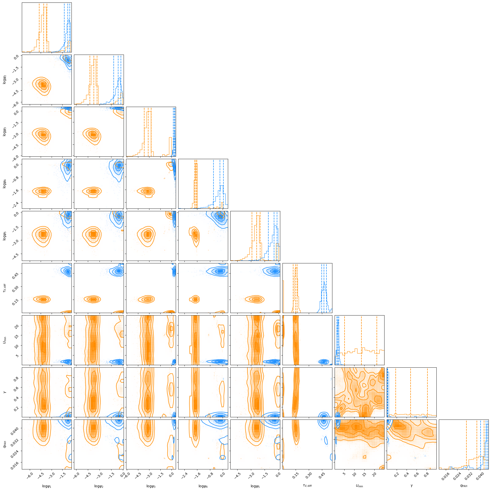
# Plot log SFH so that we can fit both
# regions on the same corner plot
tmp = samples_center[:,~const_dim]
tmp[:,:5] = np.log10(tmp[:,:5])
fig1 = corner.corner(tmp,
labels=param_labels_log[~const_dim],
quantiles=[0.16, 0.50, 0.84],
#show_titles=True,
smooth=1,
color='darkorange')
tmp = samples_disk[:,~const_dim]
tmp[:,:5] = np.log10(tmp[:,:5])
fig1 = corner.corner(tmp,
labels=param_labels_log[~const_dim],
quantiles=[0.16, 0.50, 0.84],
#show_titles=True,
smooth=1,
fig=fig1,
color='dodgerblue')
[8]:
fig3, axs = plt.subplots(9,2, figsize=(9,9))

t = 1 + np.arange(samples_center.shape[0])
for i, label in enumerate(param_labels[~const_dim]):
    axs[i,0].plot(t, samples_center[:,~const_dim][:,i], color='darkorange')
    axs[i,1].plot(t, samples_disk[:,~const_dim][:,i], color='dodgerblue')

    axs[i,0].set_ylabel(label)
    if i != 8:
        axs[i,0].set_xticklabels([])
        axs[i,1].set_xticklabels([])

    axs[i,0].set_xlim(t[0],t[-1])
    axs[i,1].set_xlim(t[0],t[-1])

axs[0,0].set_title('Center', color='darkorange')
axs[0,1].set_title('Disk', color='dodgerblue')
axs[8,0].set_xlabel('Trial Number')
axs[8,1].set_xlabel('Trial Number')
[8]:
Text(0.5, 0, 'Trial Number')
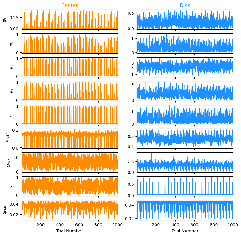
Clearly still some correlated behavior. We would need longer chains to properly converge and get a better estimate of the autocorrelation time.
[10]:
# Best-fit SED plot
fig4 = plt.figure()
ax41 = fig4.add_axes([0.1, 0.4, 0.8, 0.5])
ax42 = fig4.add_axes([0.1, 0.1, 0.8, 0.3])

# samples
# log_prob_samples

# mlgh.lnu_obs[1,:]
# mlgh.lnu_unc[1,:]
# mlgh.lnu_obs[2,:]
# mlgh.lnu_unc[2,:]
# mlgh.lnu_obs[0,:]
# mlgh.lnu_unc[0,:]

bestfit = np.argmax(log_prob_samples)
disk_lnu_best = lgh.get_model_components_lnu_hires(samples_disk[bestfit,:])
center_lnu_best = lgh.get_model_components_lnu_hires(samples_center[bestfit,:])
disk_lnu_best_total,_ = lgh.get_model_lnu_hires(samples_disk[bestfit,:])
center_lnu_best_total,_ = lgh.get_model_lnu_hires(samples_center[bestfit,:])
disk_lmod_best_total,_ = lgh.get_model_lnu(samples_disk[bestfit,:])
center_lmod_best_total,_ = lgh.get_model_lnu(samples_center[bestfit,:])
# total_total
total_lmod_best_total = disk_lmod_best_total + center_lmod_best_total

delchi_disk = (mlgh.lnu_obs[2,:] - disk_lmod_best_total) / np.sqrt(mlgh.lnu_unc[2,:]**2 + (0.10 * disk_lmod_best_total)**2)
delchi_center = (mlgh.lnu_obs[1,:] - center_lmod_best_total) / np.sqrt(mlgh.lnu_unc[1,:]**2 + (0.10 * center_lmod_best_total)**2)
delchi_unresolved = (mlgh.lnu_obs[0,:] - total_lmod_best_total) / np.sqrt(mlgh.lnu_unc[0,:]**2 + (0.10 * center_lmod_best_total)**2)

ax41.plot(lgh.wave_grid_obs,
          lgh.nu_grid_obs*disk_lnu_best_total,
          color='dodgerblue',
          label='Disk',
          alpha=0.5)
ax41.plot(lgh.wave_grid_obs,
          lgh.nu_grid_obs*center_lnu_best_total,
          color='darkorange',
          label='Center',
          alpha=0.5)
ax41.plot(lgh.wave_grid_obs,
          lgh.nu_grid_obs*(center_lnu_best_total + disk_lnu_best_total),
          color='black',
          label='Total',
          alpha=0.5)
ax41.errorbar(lgh.wave_obs,
              lgh.nu_obs * mlgh.lnu_obs[2,:],
              yerr=lgh.nu_obs * mlgh.lnu_unc[2,:],
              marker='D',
              linestyle='',
              color='dodgerblue',
              markerfacecolor='dodgerblue',
              capsize=2)
ax41.errorbar(lgh.wave_obs,
              lgh.nu_obs * mlgh.lnu_obs[1,:],
              yerr=lgh.nu_obs * mlgh.lnu_unc[1,:],
              marker='D',
              linestyle='',
              color='darkorange',
              markerfacecolor='darkorange',
              capsize=2)
ax41.errorbar(lgh.wave_obs,
              lgh.nu_obs * mlgh.lnu_obs[0,:],
              yerr=lgh.nu_obs * mlgh.lnu_unc[0,:],
              marker='D',
              linestyle='',
              color='k',
              markerfacecolor='k',
              capsize=2)

ax41.set_xscale('log')
ax41.set_yscale('log')
ax41.set_ylabel(r'$\nu L_{\nu}~[\rm L_{\odot}]$')
ax41.legend(loc='lower left')

ax42.axhline(-1, color='slategray', linestyle='--')
ax42.axhline(0, color='slategray', linestyle='-')
ax42.axhline(1, color='slategray', linestyle='--')

ax42.errorbar(lgh.wave_obs,
              delchi_disk,
              yerr=np.ones_like(delchi_disk),
              marker='D',
              color='dodgerblue',
              markerfacecolor='dodgerblue',
              linestyle='',
              capsize=2.0)
ax42.errorbar(lgh.wave_obs,
              delchi_center,
              yerr=np.ones_like(delchi_center),
              marker='D',
              color='darkorange',
              markerfacecolor='darkorange',
              linestyle='',
              capsize=2.0)
ax42.errorbar(lgh.wave_obs,
              delchi_unresolved,
              yerr=np.ones_like(delchi_unresolved),
              marker='D',
              color='k',
              markerfacecolor='k',
              linestyle='',
              capsize=2.0)
ax42.set_xscale('log')
ax42.set_xlim(ax41.get_xlim())
ax42.set_xlabel(r'Observed-Frame Wavelength [$\rm \mu m$]')
ax42.set_ylim(-5,5)
ax42.set_ylabel(r'Residual [$\sigma$]')
/Users/eqm5663/Research/code/plightning/lightning/stellar/pegase.py:443: RuntimeWarning: divide by zero encountered in log10
  finterp = interp1d(self.Zmet, np.log10(self.Lnu_obs), axis=1)
/Users/eqm5663/miniconda3_arm64/envs/ciao-4.16/lib/python3.11/site-packages/scipy/interpolate/_interpolate.py:701: RuntimeWarning: invalid value encountered in subtract
  slope = (y_hi - y_lo) / (x_hi - x_lo)[:, None]
[10]:
Text(0, 0.5, 'Residual [$\\sigma$]')
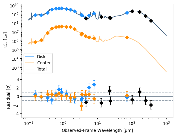
We recover a pretty decent fit, all said.
[11]:
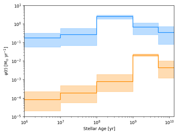
# SFH plot -- Could also normalize the SFH somehow to better show the
# differences in the shapes.
fig5, ax5 = plt.subplots()
fig5, ax5 = lgh.sfh_plot(samples_center,
                     shade_kwargs={'color':'darkorange', 'alpha':0.3, 'zorder':0},
                     line_kwargs={'color':'darkorange', 'zorder':1},
                     ax=ax5)
fig5, ax5 = lgh.sfh_plot(samples_disk,
                     shade_kwargs={'color':'dodgerblue', 'alpha':0.3, 'zorder':0},
                     line_kwargs={'color':'dodgerblue', 'zorder':1},
                     ax=ax5)

ax5.set_ylabel(r'$\psi (t)~[\rm M_{\odot}~yr^{-1}]$')
ax5.set_xlabel(r'Stellar Age [yr]')
ax5.set_xscale('log')
ax5.set_yscale('log')
ax5.set_xlim(1e6,13.6e9)
ax5.set_ylim(1e-5, 10)
[11]:
(1e-05, 10)